Tutorial
In this example we’ll classify an image with the bundled CaffeNet model (which is based on the network architecture of Krizhevsky et al. for ImageNet).
We’ll compare CPU and GPU modes and then dig into the model to inspect features and the output.
Setup
- First, set up Python,
numpy, andmatplotlib.
1 | # set up Python environment: numpy for numerical routines, and matplotlib for plotting |
CaffeNet found.
Load net and set up input preprocessing
- Set Caffe to CPU mode and load the net from disk.
1 | caffe.set_mode_cpu() |
Set up input preprocessing. (We’ll use Caffe’s
caffe.io.Transformerto do this, but this step is independent of other parts of Caffe, so any custom preprocessing code may be used).Our default CaffeNet is configured to take images in BGR format. Values are expected to start in the range [0, 255] and then have the mean ImageNet pixel value subtracted from them. In addition, the channel dimension is expected as the first (outermost) dimension.
As matplotlib will load images with values in the range [0, 1] in RGB format with the channel as the innermost dimension, we are arranging for the needed transformations here.
1 | # load the mean ImageNet image (as distributed with Caffe) for subtraction |
mean-subtracted values: [('B', 104.0069879317889), ('G', 116.66876761696767), ('R', 122.6789143406786)]
CPU classification
- Now we’re ready to perform classification. Even though we’ll only classify one image, we’ll set a batch size of 50 to demonstrate batching.
1 | # set the size of the input (we can skip this if we're happy |
- Load an image (that comes with Caffe) and perform the preprocessing we’ve set up.
1 | image = caffe.io.load_image(caffe_root + 'examples/images/cat.jpg') |
/usr/local/lib/python2.7/dist-packages/skimage/transform/_warps.py:84: UserWarning: The default mode, 'constant', will be changed to 'reflect' in skimage 0.15.
  warn("The default mode, 'constant', will be changed to 'reflect' in "


<matplotlib.image.AxesImage at 0x7f2088044450>
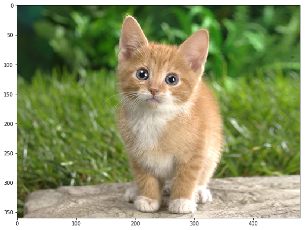
- Adorable! Let’s classify it!
1 | # copy the image data into the memory allocated for the net |
(1000,)
predicted class is: 281
- The net gives us a vector of probabilities; the most probable class was the 281st one. But is that correct? Let’s check the ImageNet labels…
1 | # load ImageNet labels |
(1000,)
output label: n02123045 tabby, tabby cat
- “Tabby cat” is correct! But let’s also look at other top (but less confident predictions).
1 | # sort top five predictions from softmax output |
probabilities and labels:


[(0.31243625, 'n02123045 tabby, tabby cat'),
 (0.23797157, 'n02123159 tiger cat'),
 (0.12387245, 'n02124075 Egyptian cat'),
 (0.10075716, 'n02119022 red fox, Vulpes vulpes'),
 (0.070957333, 'n02127052 lynx, catamount')]
- We see that less confident predictions are sensible.
Switching to GPU mode
- Let’s see how long classification took, and compare it to GPU mode.
1 | %timeit net.forward() |
1 loop, best of 3: 4.26 s per loop
- That’s a while, even for a batch of 50 images. Let’s switch to GPU mode.
1 | caffe.set_device(0) # if we have multiple GPUs, pick the first one |
10 loops, best of 3: 29.6 ms per loop
- That should be much faster!
Examining intermediate output
- A net is not just a black box; let’s take a look at some of the parameters and intermediate activations.
First we’ll see how to read out the structure of the net in terms of activation and parameter shapes.
For each layer, let’s look at the activation shapes, which typically have the form
(batch_size, channel_dim, height, width).The activations are exposed as an
OrderedDict,net.blobs.
1 | # for each layer, show the output shape |
data	(50, 3, 227, 227)
conv1	(50, 96, 55, 55)
pool1	(50, 96, 27, 27)
norm1	(50, 96, 27, 27)
conv2	(50, 256, 27, 27)
pool2	(50, 256, 13, 13)
norm2	(50, 256, 13, 13)
conv3	(50, 384, 13, 13)
conv4	(50, 384, 13, 13)
conv5	(50, 256, 13, 13)
pool5	(50, 256, 6, 6)
fc6	(50, 4096)
fc7	(50, 4096)
fc8	(50, 1000)
prob	(50, 1000)
Now look at the parameter shapes. The parameters are exposed as another
OrderedDict,net.params. We need to index the resulting values with either[0]for weights or[1]for biases.The param shapes typically have the form
(output_channels, input_channels, filter_height, filter_width)(for the weights) and the 1-dimensional shape(output_channels,)(for the biases).
1 | for layer_name, param in net.params.iteritems(): |
conv1	(96, 3, 11, 11) (96,)
conv2	(256, 48, 5, 5) (256,)
conv3	(384, 256, 3, 3) (384,)
conv4	(384, 192, 3, 3) (384,)
conv5	(256, 192, 3, 3) (256,)
fc6	(4096, 9216) (4096,)
fc7	(4096, 4096) (4096,)
fc8	(1000, 4096) (1000,)
- Since we’re dealing with four-dimensional data here, we’ll define a helper function for visualizing sets of rectangular heatmaps.
1 | def vis_square(data): |
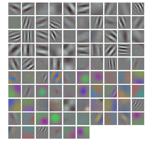
- First we’ll look at the first layer filters,
conv1
1 | # the parameters are a list of [weights, biases] |
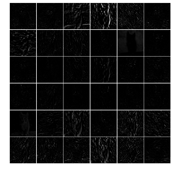
- The first layer output,
conv1(rectified responses of the filters above, first 36 only)
1 | feat = net.blobs['conv1'].data[0, :36] |
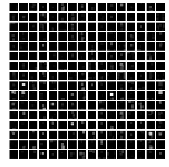
- The fifth layer after pooling,
pool5
1 | feat = net.blobs['pool5'].data[0] |
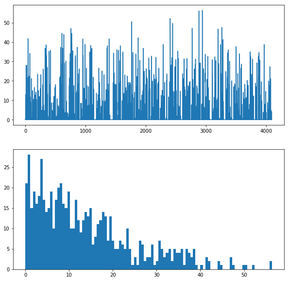
The first fully connected layer,
fc6(rectified)We show the output values and the histogram of the positive values
1 | feat = net.blobs['fc6'].data[0] |
- The final probability output,
prob
1 | feat = net.blobs['prob'].data[0] |
[<matplotlib.lines.Line2D at 0x7f2060250650>]
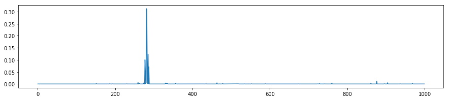
Note the cluster of strong predictions; the labels are sorted semantically. The top peaks correspond to the top predicted labels, as shown above.
Try your own image
Now we’ll grab an image from the web and classify it using the steps above.
- Try setting
my_image_urlto any JPEG image URL.
1 | # download an image |
Reference
History
- 20180807: created.