Getting Started
Shared variables tips
We encourage you to store the dataset into shared variables and access it based on the minibatch index, given a fixed and known batch size. The reason behind shared variables is related to using the GPU. There is a large overhead when copying data into the GPU memory.
将数据存储在shared variable便于加速GPU计算,避免数据从CPU拷贝到GPU。
If you have your data in Theano shared variables though, you give Theano the possibility to copy the entire data on the GPU in a single call when the shared variables are constructed.
shared构建的时候,theano一次性讲所有数据拷贝至GPU.
Because the datapoints and their labels are usually of different nature (labels are usually integers while datapoints are real numbers) we suggest to use different variables for label and data. Also we recommend using different variables for the training set, validation set and testing set to make the code more readable (resulting in 6 different shared variables).
data,label使用2个shared variables,train,valid,test使用不同的shared variables,总计6个
Mini-batch data
def shared_dataset(data_xy):
    """ Function that loads the dataset into shared variables

    The reason we store our dataset in shared variables is to allow
    Theano to copy it into the GPU memory (when code is run on GPU).
    Since copying data into the GPU is slow, copying a minibatch everytime
    is needed (the default behaviour if the data is not in a shared
    variable) would lead to a large decrease in performance.
    """
    data_x, data_y = data_xy
    shared_x = theano.shared(numpy.asarray(data_x, dtype=theano.config.floatX))
    shared_y = theano.shared(numpy.asarray(data_y, dtype=theano.config.floatX))
    # shared变量中的数据在GPU上必须是float32类型,但是计算阶段可能需要int类型(y),所以需要
    # 将float32--->int.
    # When storing data on the GPU it has to be stored as floats
    # therefore we will store the labels as ``floatX`` as well
    # (``shared_y`` does exactly that). But during our computations
    # we need them as ints (we use labels as index, and if they are
    # floats it doesn't make sense) therefore instead of returning
    # ``shared_y`` we will have to cast it to int. This little hack
    # lets us get around this issue
    return shared_x, T.cast(shared_y, 'int32')

test_set_x, test_set_y = shared_dataset(test_set)
valid_set_x, valid_set_y = shared_dataset(valid_set)
train_set_x, train_set_y = shared_dataset(train_set)

batch_size = 500    # size of the minibatch

# accessing the third minibatch of the training set

data  = train_set_x[2 * batch_size: 3 * batch_size]
label = train_set_y[2 * batch_size: 3 * batch_size]
SGD pseudo code in theano
Traditional GD (m=N)
# GRADIENT DESCENT

while True:
    loss = f(params)
    d_loss_wrt_params = ... # compute gradient
    params -= learning_rate * d_loss_wrt_params
    if <stopping condition is met>:
        return params
Stochastic gradient descent (SGD) works according to the same principles as ordinary gradient descent, but proceeds more quickly by estimating the gradient from just a few examples at a time instead of the entire training set. In its purest form, we estimate the gradient from just a single example at a time.
Online Learning SGD (m=1)
# STOCHASTIC GRADIENT DESCENT
for (x_i,y_i) in training_set:
                            # imagine an infinite generator
                            # that may repeat examples (if there is only a finite training set)
    loss = f(params, x_i, y_i)
    d_loss_wrt_params = ... # compute gradient
    params -= learning_rate * d_loss_wrt_params
    if <stopping condition is met>:
        return params
The variant that we recommend for deep learning is a further twist on stochastic gradient descent using so-called “minibatches”. Minibatch SGD (MSGD) works identically to SGD, except that we use more than one training example to make each estimate of the gradient. This technique reduces variance in the estimate of the gradient, and often makes better use of the hierarchical memory organization in modern computers.
Minibatch SGD (m)
for (x_batch,y_batch) in train_batches:
                            # imagine an infinite generator
                            # that may repeat examples
    loss = f(params, x_batch, y_batch)
    d_loss_wrt_params = ... # compute gradient using theano
    params -= learning_rate * d_loss_wrt_params
    if <stopping condition is met>:
        return params
Theano pseudo code of Minibatch SGD
# Minibatch Stochastic Gradient Descent

# assume loss is a symbolic description of the loss function given
# the symbolic variables params (shared variable), x_batch, y_batch;

# compute gradient of loss with respect to params
d_loss_wrt_params = T.grad(loss, params)

# compile the MSGD step into a theano function
updates = [(params, params - learning_rate * d_loss_wrt_params)]
MSGD = theano.function([x_batch,y_batch], loss, updates=updates)

for (x_batch, y_batch) in train_batches:
    # here x_batch and y_batch are elements of train_batches and
    # therefore numpy arrays; function MSGD also updates the params
    print('Current loss is ', MSGD(x_batch, y_batch))
    if stopping_condition_is_met:
        return params
Regularization
L1/L2 regularization
L1/L2 regularization and early-stopping.
Commonly used values for p are 1 and 2, hence the L1/L2 nomenclature. If p=2, then the regularizer is also called “weight decay”.
To follow Occam’s razor principle, this minimization should find us the simplest solution (as measured by our simplicity criterion) that fits the training data.
# symbolic Theano variable that represents the L1 regularization term
L1  = T.sum(abs(param))

# symbolic Theano variable that represents the squared L2 term
L2 = T.sum(param ** 2)

# the loss
loss = NLL + lambda_1 * L1 + lambda_2 * L2
Early-Stopping
Early-stopping combats overfitting by monitoring the model’s performance on a validation set. A validation set is a set of examples that we never use for gradient descent, but which is also not a part of the test set.
所谓early stopping,即在每一个epoch结束时(一个epoch即对所有训练数据的一轮遍历)计算 validation data的accuracy,当accuracy不再提高时,就停止训练。这是很自然的做法,因为accuracy不再提高了,训练下去也没用。另外,这样做还能防止overfitting。
那么,怎么样才算是validation accuracy不再提高呢?并不是说validation accuracy一降下来,它就是“不再提高”,因为可能经过这个epoch后,accuracy降低了,但是随后的epoch又让accuracy升上去了,所以不能根据一两次的连续降低就判断“不再提高”。正确的做法是,在训练的过程中,记录最佳的validation accuracy,当连续10次epoch(或者更多次)没达到最佳accuracy时,你可以认为“不再提高”,此时使用early stopping。这个策略就叫“ no-improvement-in-n”,n即epoch的次数,可以根据实际情况取10、20、30….
Variable learning rate
Decreasing the learning rate over time is sometimes a good idea. eta = eta0/(1+d*epoch) (d: eta decrease constant, d=0.001)
Early stopping + decrease learning rate. eta = eta0/2 until eta= eta0/1024
一个简单有效的做法就是,当validation accuracy满足 no-improvement-in-n规则时,本来我们是要early stopping的,但是我们可以不stop,而是让learning rate减半,之后让程序继续跑。下一次validation accuracy又满足no-improvement-in-n规则时,我们同样再将learning rate减半(此时变为原始learni rate的四分之一)…继续这个过程,直到learning rate变为原来的1/1024再终止程序。(1/1024还是1/512还是其他可以根据实际确定)。【PS:也可以选择每一次将learning rate除以10,而不是除以2.】
实践中,eta/2变化太快,eta0/(1+d*epoch),d=0.001比较合适。
# early-stopping parameters
patience = 5000  # look as this many examples regardless
patience_increase = 2     # wait this much longer when a new best is
                              # found
improvement_threshold = 0.995  # a relative improvement of this much is
                               # considered significant
validation_frequency = min(n_train_batches, patience/2) = 2500 # for iters
                              # go through this many
                              # minibatches before checking the network
                              # on the validation set; in this case we
                              # check every epoch

best_params = None
best_validation_loss = numpy.inf
test_score = 0.
start_time = time.clock()

done_looping = False
epoch = 0
while (epoch < n_epochs) and (not done_looping):
    # Report "1" for first epoch, "n_epochs" for last epoch
    epoch = epoch + 1
    for minibatch_index in range(n_train_batches):

        d_loss_wrt_params = ... # compute gradient
        params -= learning_rate * d_loss_wrt_params # gradient descent

        # iteration number. We want it to start at 0.
        iter = (epoch - 1) * n_train_batches + minibatch_index
        # note that if we do `iter % validation_frequency` it will be
        # true for iter = 0 which we do not want. We want it true for
        # iter = validation_frequency - 1.
        if (iter + 1) % validation_frequency == 0:

            this_validation_loss = ... # compute zero-one loss on validation set

            if this_validation_loss < best_validation_loss:

                # improve patience if loss improvement is good enough
                if this_validation_loss < best_validation_loss * improvement_threshold:
                    patience = max(patience, iter * patience_increase)

                best_params = copy.deepcopy(params)
                best_validation_loss = this_validation_loss

        if patience <= iter:
            done_looping = True
            break

# POSTCONDITION:
# best_params refers to the best out-of-sample parameters observed during the optimization
Theano/Python Tips
Loading and Saving Models
DO: Pickle the numpy ndarrays from your shared variables
DON’T: Do not pickle your training or test functions for long-term storage
import cPickle
save_file = open('path', 'wb')  # this will overwrite current contents
cPickle.dump(w.get_value(borrow=True), save_file, -1)  # the -1 is for HIGHEST_PROTOCOL
cPickle.dump(v.get_value(borrow=True), save_file, -1)  # .. and it triggers much more efficient
cPickle.dump(u.get_value(borrow=True), save_file, -1)  # .. storage than numpy's default
save_file.close()
Then later, you can load your data back like this:
save_file = open('path')
w.set_value(cPickle.load(save_file), borrow=True)
v.set_value(cPickle.load(save_file), borrow=True)
u.set_value(cPickle.load(save_file), borrow=True)
Plotting Intermediate Results
If you have enough disk space, your training script should save intermediate models and a visualization script should process those saved models.
MLP
see here
An MLP can be viewed as a logistic regression classifier where the input is first transformed using a learnt non-linear transformation sigmoid. This transformation projects the input data into a space where it becomes linearly separable. This intermediate layer is referred to as a hidden layer. A single hidden layer is sufficient to make MLPs a universal approximator.
weight initializations
- old version: 1/sqrt(n_in)
The initial values for the weights of a hidden layer i should be uniformly sampled from a symmetric interval that depends on the activation function. weight的初始化依赖于activation
- tanh: uniformely sampled from -sqrt(6./(n_in+n_hidden)) and sqrt(6./(n_in+n_hidden))
- sigmoid : use 4 times larger initial weights for sigmoid compared to tanh
# `W` is initialized with `W_values` which is uniformely sampled
        # from sqrt(-6./(n_in+n_hidden)) and sqrt(6./(n_in+n_hidden))
        # for tanh activation function
        # the output of uniform if converted using asarray to dtype
        # theano.config.floatX so that the code is runable on GPU
        # Note : optimal initialization of weights is dependent on the
        #        activation function used (among other things).
        #        For example, results presented in [Xavier10] suggest that you
        #        should use 4 times larger initial weights for sigmoid
        #        compared to tanh
        #        We have no info for other function, so we use the same as
        #        tanh.
        if W is None:
            W_values = numpy.asarray(
                rng.uniform(
                    low=-numpy.sqrt(6. / (n_in + n_out)),
                    high=numpy.sqrt(6. / (n_in + n_out)),
                    size=(n_in, n_out)
                ),
                dtype=theano.config.floatX
            )
            if activation == theano.tensor.nnet.sigmoid:
                W_values *= 4

            W = theano.shared(value=W_values, name='W', borrow=True)

        if b is None:
            b_values = numpy.zeros((n_out,), dtype=theano.config.floatX)
            b = theano.shared(value=b_values, name='b', borrow=True)

        self.W = W
        self.b = b
Tips and Tricks for training MLPs
Nonlinearity
Two of the most common ones are the sigmoid and the tanh function. nonlinearities that are symmetric around the origin are preferred because they tend to produce zero-mean inputs to the next layer (which is a desirable property). Empirically, we have observed that the tanh has better convergence properties.
Weight initialization
At initialization we want the weights to be small enough around the origin so that the activation function operates in its linear regime, where gradients are the largest. weight的初始化依赖于activation
Learning rate
The simplest solution is to simply have a constant rate. Rule of thumb: try several log-spaced values (10^{-1},10^{-2},\ldots) and narrow the (logarithmic) grid search to the region where you obtain the lowest validation error.
Decreasing the learning rate over time is sometimes a good idea. eta = eta0/(1+d*epoch) (d: decrease constant, 0.001)
Early stopping + decrease learning rate. eta = eta0/2 until eta= eta0/1024
Regularization parameter
Typical values to try for the L1/L2 regularization parameter \lambda are 10^{-2},10^{-3},\ldots. In the framework that we described so far, optimizing this parameter will not lead to significantly better solutions, but is worth exploring nonetheless.
Number of hidden units
This hyper-parameter is very much dataset-dependent. hidden neurons的数量依赖于具体的数据集。Unless we employ some regularization scheme (early stopping or L1/L2 penalties), a typical number of hidden units vs. generalization performance graph will be U-shaped.
CNN
The Convolution and Pool Operator
import theano
from theano import tensor as T
from theano.tensor.nnet import conv2d,sigmoid
from theano.tensor.signal.pool import pool_2d
import numpy
import numpy as np
import matplotlib.pyplot as plt
from PIL import Image
rng = numpy.random.RandomState(23455)
# instantiate 4D tensor for input
input = T.tensor4(name='input')
# initialize shared variable for weights.
w_shp = (2, 3, 9, 9)
w_bound = numpy.sqrt(3 * 9 * 9)
W = theano.shared( numpy.asarray(
rng.uniform(
low=-1.0 / w_bound,
high=1.0 / w_bound,
size=w_shp),
dtype=input.dtype), name ='W')
# initialize shared variable for bias (1D tensor) with random values
# IMPORTANT: biases are usually initialized to zero. However in this
# particular application, we simply apply the convolutional layer to
# an image without learning the parameters. We therefore initialize
# them to random values to "simulate" learning.
b_shp = (2,)
b = theano.shared(numpy.asarray(
rng.uniform(low=-.5, high=.5, size=b_shp),
dtype=input.dtype), name ='b')
# build symbolic expression that computes the convolution of input with filters in w
conv_out = conv2d(input, W)
poolsize=(2,2)
pooled_out = pool_2d( input=conv_out, ws=poolsize, ignore_border=True)
conv_activations = sigmoid(conv_out + b.dimshuffle('x', 0, 'x', 'x'))
# create theano function to compute filtered images
f = theano.function([input], conv_activations)
pooled_activations = sigmoid(pooled_out + b.dimshuffle('x', 0, 'x', 'x'))
f2 = theano.function([input], pooled_activations)
#===========================================================
# processing image file
#===========================================================
# open random image of dimensions 639x516
img = Image.open(open('./3wolfmoon.jpg'))
# dimensions are (height, width, channel)
img = numpy.asarray(img, dtype=theano.config.floatX) / 256.
# put image in 4D tensor of shape (1, 3, height, width)
input_img_ = img.transpose(2, 0, 1).reshape(1, 3, 639, 516)
filtered_img = f(input_img_)
pooled_img = f2(input_img_)
print filtered_img.shape # (1, 2, 631, 508) 2 feature maps
print pooled_img.shape # (1, 2, 315, 254) 2 feature maps
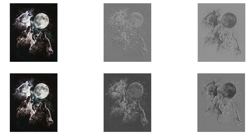
fig = plt.figure(figsize=(16,8))
# (1)
# plot original image and first and second components of output
plt.subplot(2, 3, 1); plt.axis('off'); plt.imshow(img)
plt.gray();
# recall that the convOp output (filtered image) is actually a "minibatch",
# of size 1 here, so we take index 0 in the first dimension:
plt.subplot(2, 3, 2); plt.axis('off'); plt.imshow(filtered_img[0, 0, :, :])
plt.subplot(2, 3, 3); plt.axis('off'); plt.imshow(filtered_img[0, 1, :, :])
# (2)
# plot original image and first and second components of output
plt.subplot(2, 3, 4); plt.axis('off'); plt.imshow(img)
plt.gray();
# recall that the convOp output (filtered image) is actually a "minibatch",
# of size 1 here, so we take index 0 in the first dimension:
plt.subplot(2, 3, 5); plt.axis('off'); plt.imshow(pooled_img[0, 0, :, :])
plt.subplot(2, 3, 6); plt.axis('off'); plt.imshow(pooled_img[0, 1, :, :])
plt.show()
# Notice that a randomly initialized filter acts very much like an edge detector!
WARNING (theano.sandbox.cuda): The cuda backend is deprecated and will be removed in the next release (v0.10).  Please switch to the gpuarray backend. You can get more information about how to switch at this URL:
 https://github.com/Theano/Theano/wiki/Converting-to-the-new-gpu-back-end%28gpuarray%29

Using gpu device 0: GeForce GTX 1060 (CNMeM is enabled with initial size: 80.0% of memory, cuDNN 5105)


(1, 2, 631, 508)
(1, 2, 315, 254)
Reference
History
- 20180807: created.