Tutorial

In this tutorial we will do multilabel classification on PASCAL VOC 2012.

Multilabel classification is a generalization of multiclass classification, where each instance (image) can belong to many classes. For example, an image may both belong to a “beach” category and a “vacation pictures” category. In multiclass classification, on the other hand, each image belongs to a single class.

Caffe supports multilabel classification through the SigmoidCrossEntropyLoss layer, and we will load data using a Python data layer. Data could also be provided through HDF5 or LMDB data layers, but the python data layer provides endless flexibility, so that’s what we will use.

Preliminaries

First, make sure you compile caffe using
WITH_PYTHON_LAYER := 1
Second, download PASCAL VOC 2012. It’s available here:
Third, import modules:

import sys 
import os

import numpy as np
import os.path as osp
import matplotlib.pyplot as plt

from copy import copy

% matplotlib inline
plt.rcParams['figure.figsize'] = (6, 6)

caffe_root = '../'  # this file is expected to be in {caffe_root}/examples
sys.path.append(caffe_root + 'python')
import caffe # If you get "No module named _caffe", either you have not built pycaffe or you have the wrong path.

from caffe import layers as L, params as P # Shortcuts to define the net prototxt.

sys.path.append("pycaffe/layers") # the datalayers we will use are in this directory.
sys.path.append("pycaffe") # the tools file is in this folder

import tools #this contains some tools that we need

Fourth, set data directories and initialize caffe

# set data root directory, e.g:
pascal_root = osp.join(caffe_root, 'data/pascal/VOC2012')

# these are the PASCAL classes, we'll need them later.
classes = np.asarray(['aeroplane', 'bicycle', 'bird', 'boat', 'bottle', 
                      'bus', 'car', 'cat', 'chair', 'cow', 'diningtable',
                      'dog', 'horse', 'motorbike', 'person', 'pottedplant', 
                      'sheep', 'sofa', 'train', 'tvmonitor'])

# make sure we have the caffenet weight downloaded.
#if not os.path.isfile(caffe_root + 'models/bvlc_reference_caffenet/bvlc_reference_caffenet.caffemodel'):
#    print("Downloading pre-trained CaffeNet model...")
#    !../scripts/download_model_binary.py ../models/bvlc_reference_caffenet

# initialize caffe for gpu mode
caffe.set_mode_gpu()
caffe.set_device(0)

Define network prototxts

Let’s start by defining the nets using caffe.NetSpec. Note how we used the SigmoidCrossEntropyLoss layer. This is the right loss for multilabel classification. Also note how the data layer is defined.

# helper function for common structures
def conv_relu(bottom, ks, nout, stride=1, pad=0, group=1):
    conv = L.Convolution(bottom, kernel_size=ks, stride=stride,
                                num_output=nout, pad=pad, group=group)
    return conv, L.ReLU(conv, in_place=True)

# another helper function
def fc_relu(bottom, nout):
    fc = L.InnerProduct(bottom, num_output=nout)
    return fc, L.ReLU(fc, in_place=True)

# yet another helper function
def max_pool(bottom, ks, stride=1):
    return L.Pooling(bottom, pool=P.Pooling.MAX, kernel_size=ks, stride=stride)

# main netspec wrapper
def caffenet_multilabel(data_layer_params, datalayer):
    # setup the python data layer 
    n = caffe.NetSpec()
    n.data, n.label = L.Python(module = 'pascal_multilabel_datalayers', layer = datalayer, 
                               ntop = 2, param_str=str(data_layer_params))

    # the net itself
    n.conv1, n.relu1 = conv_relu(n.data, 11, 96, stride=4)
    n.pool1 = max_pool(n.relu1, 3, stride=2)
    n.norm1 = L.LRN(n.pool1, local_size=5, alpha=1e-4, beta=0.75)
    n.conv2, n.relu2 = conv_relu(n.norm1, 5, 256, pad=2, group=2)
    n.pool2 = max_pool(n.relu2, 3, stride=2)
    n.norm2 = L.LRN(n.pool2, local_size=5, alpha=1e-4, beta=0.75)
    n.conv3, n.relu3 = conv_relu(n.norm2, 3, 384, pad=1)
    n.conv4, n.relu4 = conv_relu(n.relu3, 3, 384, pad=1, group=2)
    n.conv5, n.relu5 = conv_relu(n.relu4, 3, 256, pad=1, group=2)
    n.pool5 = max_pool(n.relu5, 3, stride=2)
    n.fc6, n.relu6 = fc_relu(n.pool5, 4096)
    n.drop6 = L.Dropout(n.relu6, in_place=True)
    n.fc7, n.relu7 = fc_relu(n.drop6, 4096)
    n.drop7 = L.Dropout(n.relu7, in_place=True)
    n.score = L.InnerProduct(n.drop7, num_output=20) # z value
    n.loss = L.SigmoidCrossEntropyLoss(n.score, n.label) # a = sigmoid(z)

    return str(n.to_proto())

Write nets and solver files

Now we can crete net and solver prototxts. For the solver, we use the CaffeSolver class from the “tools” module

workdir = './pascal_multilabel_with_datalayer'
if not os.path.isdir(workdir):
    os.makedirs(workdir)

solverprototxt = tools.CaffeSolver(trainnet_prototxt_path = osp.join(workdir, "trainnet.prototxt"), 
                                   testnet_prototxt_path = osp.join(workdir, "valnet.prototxt"))
solverprototxt.sp['display'] = "1"
solverprototxt.sp['base_lr'] = "0.0001"
solverprototxt.write(osp.join(workdir, 'solver.prototxt'))

# write train net.
with open(osp.join(workdir, 'trainnet.prototxt'), 'w') as f:
    # provide parameters to the data layer as a python dictionary. Easy as pie!
    data_layer_params = dict(batch_size = 128, im_shape = [227, 227], split = 'train', pascal_root = pascal_root)
    f.write(caffenet_multilabel(data_layer_params, 'PascalMultilabelDataLayerSync'))

# write validation net.
with open(osp.join(workdir, 'valnet.prototxt'), 'w') as f:
    data_layer_params = dict(batch_size = 128, im_shape = [227, 227], split = 'val', pascal_root = pascal_root)
    f.write(caffenet_multilabel(data_layer_params, 'PascalMultilabelDataLayerSync'))

This net uses a python datalayer: ‘PascalMultilabelDataLayerSync’, which is defined in ‘./pycaffe/layers/pascal_multilabel_datalayers.py’.
Take a look at the code. It’s quite straight-forward, and gives you full control over data and labels.
Now we can load the caffe solver as usual.

solver = caffe.SGDSolver(osp.join(workdir, 'solver.prototxt'))
solver.net.copy_from(caffe_root + 'models/bvlc_reference_caffenet/bvlc_reference_caffenet.caffemodel')
solver.test_nets[0].share_with(solver.net)
solver.step(1) # load 128 train images
# 5717 train images; 5823 val images

BatchLoader initialized with 5717 images
PascalMultilabelDataLayerSync initialized for split: train, with bs: 128, im_shape: [227, 227].
BatchLoader initialized with 5823 images
PascalMultilabelDataLayerSync initialized for split: val, with bs: 128, im_shape: [227, 227].

print solver.net.blobs['data'].data.shape # (128, 3, 227, 227)
print solver.net.blobs['label'].data.shape # (128, 20)

#print solver.net.blobs['loss'].data   # 13.8629436493
#print solver.test_nets[0].blobs['data'].data.shape # (128, 3, 227, 227) no test images loaded

#print solver.net.params['score'][0].data.shape # (20, 4096)  filled weights
#print solver.net.params['score'][0].data[:20,:5]

(128, 3, 227, 227)
(128, 20)

Let’s check the data we have loaded.

transformer = tools.SimpleTransformer() # This is simply to add back the bias, re-shuffle the color channels to RGB, and so on...
image_index = 0 # First image in the batch.
image = solver.net.blobs['data'].data[image_index, ...]
print image.shape # (3, 227, 227) BGR [0,255]
#print image[0,:10,:10]

plot_image = transformer.deprocess(copy(image))
#print plot_image.shape #(227, 227, 3) RGB [0,255]
#print plot_image[:10,:10,0]

image_labels = solver.net.blobs['label'].data[image_index]
print image_labels.shape # (20,)
print image_labels #float32 [ 0.  0.  0.  0.  0.  0.  0.  0.  0.  0.  0.  0.  1.  0.  1.  0.  0.  0.  0.  0.]

plt.figure()
plt.imshow(plot_image)
gtlist = image_labels.astype(np.int) # float32->int labels
plt.title('GT: {}'.format(classes[np.where(gtlist)])) # ground truth label list
plt.axis('off')

(3, 227, 227)
(20,)
[ 0.  0.  0.  0.  0.  0.  0.  0.  0.  0.  0.  0.  1.  0.  1.  0.  0.  0.
  1.  0.]

png

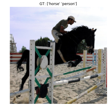
NOTE: we are readin the image from the data layer, so the resolution is lower than the original PASCAL image.

Train a net

Let’s train the net. First, though, we need some way to measure the accuracy. Hamming distance is commonly used in multilabel problems. We also need a simple test loop. Let’s write that down.

def hamming_distance(gt, est):
    # accu for only one image
    #   gt(20,) [0 0 0 0 0 0 0 0 0 0 0 0 0 0 0 0 0 0 1 1]
    #  est(20,) [0 0 0 0 0 0 0 0 0 0 0 0 0 0 0 0 0 1 1 1]
    # accu = 19/20 = 0.95
    #print gt.shape,est.shape
    return sum([1 for (g, e) in zip(gt, est) if g == e]) / float(len(gt))

def check_accuracy(net, num_batches, batch_size = 128):
    acc = 0.0
    for t in range(num_batches):
        net.forward() # load 128 batch images from test_nets
        gts = net.blobs['label'].data # (128,20)
        gts = gts.astype(np.int) # float32->int

        ests = net.blobs['score'].data > 0 # (128,20)  z-score>0===>1,otherwise ===>0
        ests = ests.astype(np.int) # bool->int

        for gt, est in zip(gts, ests): #for each ground truth and estimated label vector
            acc += hamming_distance(gt, est) # gt(20,) est(20,) for 1 image
    return acc / (num_batches * batch_size)

Alright, now let’s train for a while

%%time
for itt in range(6):
    solver.step(100)
    print 'itt:{:3d}'.format((itt + 1) * 100), 'accuracy:{0:.4f}'.format(check_accuracy(solver.test_nets[0], 50))

#itt:100 accuracy:0.9591
#itt:200 accuracy:0.9599
#itt:300 accuracy:0.9596
#itt:400 accuracy:0.9584
#itt:500 accuracy:0.9598
#itt:600 accuracy:0.9590

itt:100 accuracy:0.9591
itt:200 accuracy:0.9599
itt:300 accuracy:0.9596
itt:400 accuracy:0.9584
itt:500 accuracy:0.9598
itt:600 accuracy:0.9590

Great, the accuracy is increasing, and it seems to converge rather quickly. It may seem strange that it starts off so high but it is because the ground truth is sparse. There are 20 classes in PASCAL, and usually only one or two is present. So predicting all zeros yields rather high accuracy. Let’s check to make sure.

%%time
num_train_images = 5717
num_val_images = 5823
num_batches = num_val_images/128 # 45

def check_baseline_accuracy(net, num_batches, batch_size = 128):
    acc = 0.0
    for t in range(num_batches):
        net.forward()
        gts = net.blobs['label'].data        # (128,20)  labels
        ests = np.zeros((batch_size, 20))       # (128,20)  set to [0,0,0,...0,0]
        for gt, est in zip(gts, ests): #for each ground truth and estimated label vector
            acc += hamming_distance(gt, est)
    return acc / (num_batches * batch_size)

# gts 19 + 1, est 20, accu = 19/20 = 0.95
# gts 18 + 2, est 20, accu = 18/20 = 0.90
# avg cases: 0.925
print 'Baseline accuracy:{0:.4f}'.format(check_baseline_accuracy(solver.test_nets[0], num_batches))

Baseline accuracy:0.9241
CPU times: user 40.4 s, sys: 864 ms, total: 41.3 s
Wall time: 41.3 s

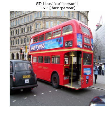
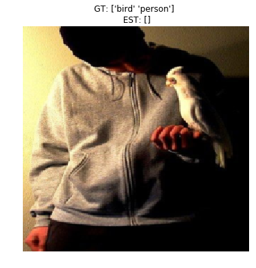
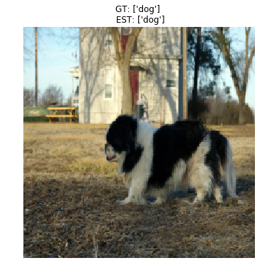
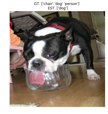
Look at some prediction results

test_net = solver.test_nets[0]
print classes
for image_index in range(5):
    print 
    plt.figure()
    plot_image = transformer.deprocess(copy(test_net.blobs['data'].data[image_index,...]))
    plt.imshow(plot_image)
    gtlist = test_net.blobs['label'].data[image_index, ...].astype(np.int)
    print 'gt',gtlist
    estlist = test_net.blobs['score'].data[image_index, ...] > 0
    estlist = estlist.astype(np.int)
    print 'est',estlist
    plt.title('GT: {} \n EST: {}'.format(classes[np.where(gtlist)], classes[np.where(estlist)]))
    plt.axis('off')

['aeroplane' 'bicycle' 'bird' 'boat' 'bottle' 'bus' 'car' 'cat' 'chair'
 'cow' 'diningtable' 'dog' 'horse' 'motorbike' 'person' 'pottedplant'
 'sheep' 'sofa' 'train' 'tvmonitor']

gt [0 0 0 0 0 1 1 0 0 0 0 0 0 0 1 0 0 0 0 0]
est [0 0 0 0 0 1 0 0 0 0 0 0 0 0 1 0 0 0 0 0]

gt [0 0 0 0 0 0 0 1 0 0 0 0 0 0 0 0 0 0 0 0]
est [0 0 0 0 0 0 0 1 0 0 0 0 0 0 0 0 0 0 0 0]

gt [0 0 1 0 0 0 0 0 0 0 0 0 0 0 1 0 0 0 0 0]
est [0 0 0 0 0 0 0 0 0 0 0 0 0 0 0 0 0 0 0 0]

gt [0 0 0 0 0 0 0 0 0 0 0 1 0 0 0 0 0 0 0 0]
est [0 0 0 0 0 0 0 0 0 0 0 1 0 0 0 0 0 0 0 0]

gt [0 0 0 0 0 0 0 0 1 0 0 1 0 0 1 0 0 0 0 0]
est [0 0 0 0 0 0 0 0 0 0 0 1 0 0 0 0 0 0 0 0]

png